Calculate the Kaplan-Meier estimator and the Aalen-Johansen estimator

Core estimation routine that computes a survfit-compatible object from a formula + data interface (Event() or survival::Surv() on the LHS, and a stratification variable on the RHS if necessary). The back-end C++ routine supports both weighted and stratified data. Use this when you want numbers only (e.g. estimates, SEs, CIs and influence functions) and will plot it yourself.

Usage

cifcurve(
  formula,
  data,
  weights = NULL,
  n.risk.type = "weighted",
  subset.condition = NULL,
  na.action = na.omit,
  outcome.type = NULL,
  time.point = NULL,
  null.hypothesis = NULL,
  code.event1 = 1,
  code.event2 = 2,
  code.censoring = 0,
  error = NULL,
  conf.type = "arcsine-square root",
  conf.int = 0.95,
  report.influence.function = FALSE,
  report.survfit.std.err = FALSE,
  engine = "calculateAJ_Rcpp",
  prob.bound = 1e-07
)

Arguments

formula: A model formula specifying the time-to-event outcome on the LHS (typically Event(time, status) or survival::Surv(time, status)) and, optionally, a stratification variable on the RHS. Unlike cifplot(), this function does not accept a fitted survfit object.
data: A data frame containing variables in the formula.
weights: Optional name of the weight variable in data. Weights must be nonnegative.
n.risk.type: Character string; one of "weighted", "unweighted", or "ess". Controls which risk set size is returned in $n.risk without affecting estimates or SEs (default "weighted").
subset.condition: Optional character string giving a logical condition to subset data (default NULL).
na.action: A function specifying the action to take on missing values (default na.omit).
outcome.type: Character string specifying the type of time-to-event outcome. One of "survival" (Kaplan-Meier) or "competing-risk" (Aalen-Johansen). If NULL (default), the function automatically infers the outcome type from the data: if the event variable has more than two unique levels, "competing-risk" is assumed; otherwise, "survival" is used. You can also use abbreviations such as "S" or "C". Mixed or ambiguous inputs (e.g., c("S", "C")) trigger automatic detection based on the event coding.
time.point: Optional single time point at which a one-sided normal approximation test is performed when null.hypothesis is specified.
null.hypothesis: Optional null value for the survival probability or cumulative incidence at time.point. For outcome.type = "survival", the one-sided alternative is that the observed survival probability is higher than the null value. For outcome.type = "competing-risk", the one-sided alternative is that the observed CIF for code.event1 is lower than the null value. A scalar value is recycled across strata. A named numeric vector can be used to specify stratum-specific null values.
code.event1: Integer code of the event of interest (default 1).
code.event2: Integer code of the competing risk (default 2).
code.censoring: Integer code of censoring (default 0).
error: Character string specifying the method for SEs and CIs used internally. For "survival" without weights, choose one of "greenwood" (default), "tsiatis", or "if". For "competing-risk" without weights, choose one of "delta" (default), "aalen", or "if". SEs and CIs based on influence functions ("if") is recommended for weighted analysis.
conf.type: Character specifying the method of transformation for CIs used internally (default arcsine-square root).
conf.int: Numeric two-sided level of CIs (default 0.95).
report.influence.function: Logical. When TRUE and engine = "calculateAJ_Rcpp", the influence function is also computed and returned (default FALSE).
report.survfit.std.err: Logical. If TRUE, report SE on the log-survival scale (survfit's convention). Otherwise SE is on the probability scale.
engine: Character. One of "auto", "calculateKM", or "calculateAJ_Rcpp" (default "calculateAJ_Rcpp").
prob.bound: Numeric lower bound used to internally truncate probabilities away from 0 and 1 (default 1e-7).

Value

A "survfit" object. For outcome.type="survival", $surv is the survival function. For outcome.type="competing-risk", $surv equals 1 - CIF for code.event1. SE and CIs are provided per error, conf.type and conf.int. This enables an independent use of standard methods for survfit such as:

summary(): time-by-time estimates with SEs and CIs
plot(): base R stepwise survival/CIF curves
mean(): restricted mean survival estimates with CIs
quantile(): quantile estimates with CIs

If null.hypothesis is specified, the returned object additionally contains a one.sided.p list with the one-sided normal approximation test results.

Note that $n.risk, $n.event, and $n.censor are rounded up to the nearest integer regardless of whether the data is weighted or not. Some methods (e.g. residuals.survfit) may not be supported.

Details

Typical use cases

When outcome.type = "survival", this is a thin wrapper around the KM estimator with the chosen variance / CI transformation.
When outcome.type = "competing-risk", this computes the AJ estimator of CIF for code.event1. The returned $surv is 1 - CIF, i.e. in the format that ggsurvfit expects.
Use cifplot() if you want to go straight to a figure; use cifcurve() if you only want the numbers.

Risk set display

Set n.risk.type to control whether $n.risk reflects weighted, unweighted, or Kish effective sample size (ESS) counts. This only affects the reported counts (e.g., for plotting or debugging) and leaves estimates and SEs unchanged.

Standard error and confidence intervals

Argument	Description	Default
`error`	SE for KM: `"greenwood"`, `"tsiatis"`, `"if"`. For CIF: `"aalen"`, `"delta"`, `"if"`.	`"greenwood"`, `"delta"` or `"if"`
`conf.type`	Transformation for CIs: `"plain"`, `"log"`, `"log-log"`, `"arcsin"`, `"logit"`, or `"none"`.	`"arcsin"`
`conf.int`	Two-sided CI level.	`0.95`

One-sided normal approximation test

When both time.point and null.hypothesis are specified, cifcurve() compares the estimate at time.point with null.hypothesis using a normal approximation. The test statistic is $$ Z = (g(\hat{p}) - g(p_0)) / \widehat{SE}(g(\hat{p})). $$ where g() is the transformation specified by conf.type. For survival outcomes, $\hat p$ is the Kaplan-Meier survival estimate and the default one-sided alternative is $S(t) > S_0(t)$. For competing-risk outcomes, the reported estimate is the Aalen-Johansen cumulative incidence estimate $F_1(t)$ for code.event1, but the transformation for the one-sided test is applied to $1 - F_1(t)$ and $1 - F_{10}(t)$, consistently with the survfit-compatible $surv component. Thus, conf.type = "log-log" corresponds to $\log[-\log(1 - F_1(t))]$ for competing-risk outcomes. The default one-sided alternative is $F_1(t) < F_{10}(t)$, equivalently $1 - F_1(t) > 1 - F_{10}(t)$. When strata are present, the test is calculated separately within each stratum.

Lifecycle

Examples

data(diabetes.complications)
output1 <- cifcurve(Event(t,epsilon) ~ fruitq,
                    data = diabetes.complications,
                    outcome.type="competing-risk")
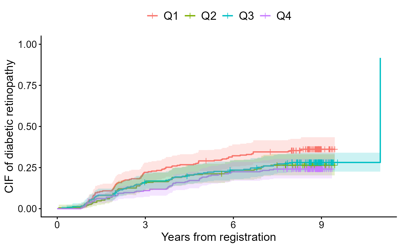
cifplot(output1,
        outcome.type = "competing-risk",
        type.y = "risk",
        add.risktable = FALSE,
        label.y = "CIF of diabetic retinopathy",
        label.x = "Years from registration")


output2 <- cifcurve(Event(t,epsilon) ~ fruitq,
                    data = diabetes.complications,
                    outcome.type = "competing-risk",
                    time.point = 8,
                    null.hypothesis = 0.30)
#> 
#> One-sided normal approximation test
#> Alternative: observed cumulative incidence is lower than null.hypothesis
#> Time point: 8
#> Transformation: arcsine-square root
#>     strata time.point        estimate.type  estimate null.hypothesis    std.err
#>  fruitq=Q1          8 cumulative incidence 0.3531391             0.3 0.03578625
#>  fruitq=Q2          8 cumulative incidence 0.2643748             0.3 0.03298645
#>  fruitq=Q3          8 cumulative incidence 0.2811656             0.3 0.02943527
#>  fruitq=Q4          8 cumulative incidence 0.2408163             0.3 0.03032340
#>      transformation.scale estimate.for.test null.for.test estimate.transformed
#>  1 - cumulative incidence         0.6468609           0.7            0.9344572
#>  1 - cumulative incidence         0.7356252           0.7            1.0307521
#>  1 - cumulative incidence         0.7188344           0.7            1.0119003
#>  1 - cumulative incidence         0.7591837           0.7            1.0578685
#>  null.transformed std.err.transformed          z    p.value
#>         0.9911566          0.03743759 -1.5145047 0.93505106
#>         0.9911566          0.03739962  1.0587137 0.14486509
#>         0.9911566          0.03273727  0.6336425 0.26315707
#>         0.9911566          0.03545942  1.8813595 0.02996152
output2$one.sided.p
#> $method
#> [1] "One-sided normal approximation test"
#> 
#> $outcome.type
#> [1] "competing-risk"
#> 
#> $alternative
#> [1] "observed cumulative incidence is lower than null.hypothesis"
#> 
#> $conf.type
#> [1] "arcsine-square root"
#> 
#> $time.point
#> [1] 8
#> 
#> $table
#>      strata time.point        estimate.type  estimate null.hypothesis
#> 1 fruitq=Q1          8 cumulative incidence 0.3531391             0.3
#> 2 fruitq=Q2          8 cumulative incidence 0.2643748             0.3
#> 3 fruitq=Q3          8 cumulative incidence 0.2811656             0.3
#> 4 fruitq=Q4          8 cumulative incidence 0.2408163             0.3
#>      std.err     transformation.scale estimate.for.test null.for.test
#> 1 0.03578625 1 - cumulative incidence         0.6468609           0.7
#> 2 0.03298645 1 - cumulative incidence         0.7356252           0.7
#> 3 0.02943527 1 - cumulative incidence         0.7188344           0.7
#> 4 0.03032340 1 - cumulative incidence         0.7591837           0.7
#>   estimate.transformed null.transformed std.err.transformed          z
#> 1            0.9344572        0.9911566          0.03743759 -1.5145047
#> 2            1.0307521        0.9911566          0.03739962  1.0587137
#> 3            1.0119003        0.9911566          0.03273727  0.6336425
#> 4            1.0578685        0.9911566          0.03545942  1.8813595
#>      p.value
#> 1 0.93505106
#> 2 0.14486509
#> 3 0.26315707
#> 4 0.02996152
#>