Example 1. Unadjusted competing risks analysis
For the initial illustration, unadjusted analysis focusing on
cumulative incidence of diabetic retinopathy (event 1) and macrovascular
complications (event 2) at 8 years of follow-up is demonstrated.
To visualize each stratification variable separately,
set panel.per.variable = TRUE. Each variable on the
right-hand side is plotted in its own panel, and the layout can be
controlled with rows.columns.panel. The figure below
contrasts the cumulative incidence curves of diabetic retinopathy for
the quartiles fruitq and a binary exposure
fruitq1, low (Q1) and high (Q2 to 4) intake of fruit,
generated by cifplot(). The add.conf=TRUE
argument adds confidence intervals to the plot. This helps visualize the
statistical uncertainty of estimated probabilities across exposure
levels. When using s continuous variable for stratification, discretize
them beforehand with cut() or factor(). The
labels of x-axis (Time) and y-axis (Cumulative incidence) in these
panels are default labels.
data(diabetes.complications)
diabetes.complications$fruitq1 <- ifelse(
  diabetes.complications$fruitq == "Q1","Q1","Q2 to Q4"
)
cifplot(Event(t,epsilon)~fruitq+fruitq1, data=diabetes.complications,
        outcome.type="competing-risk",
        add.conf=TRUE, add.censor.mark=FALSE,
        add.competing.risk.mark=FALSE, panel.per.variable=TRUE)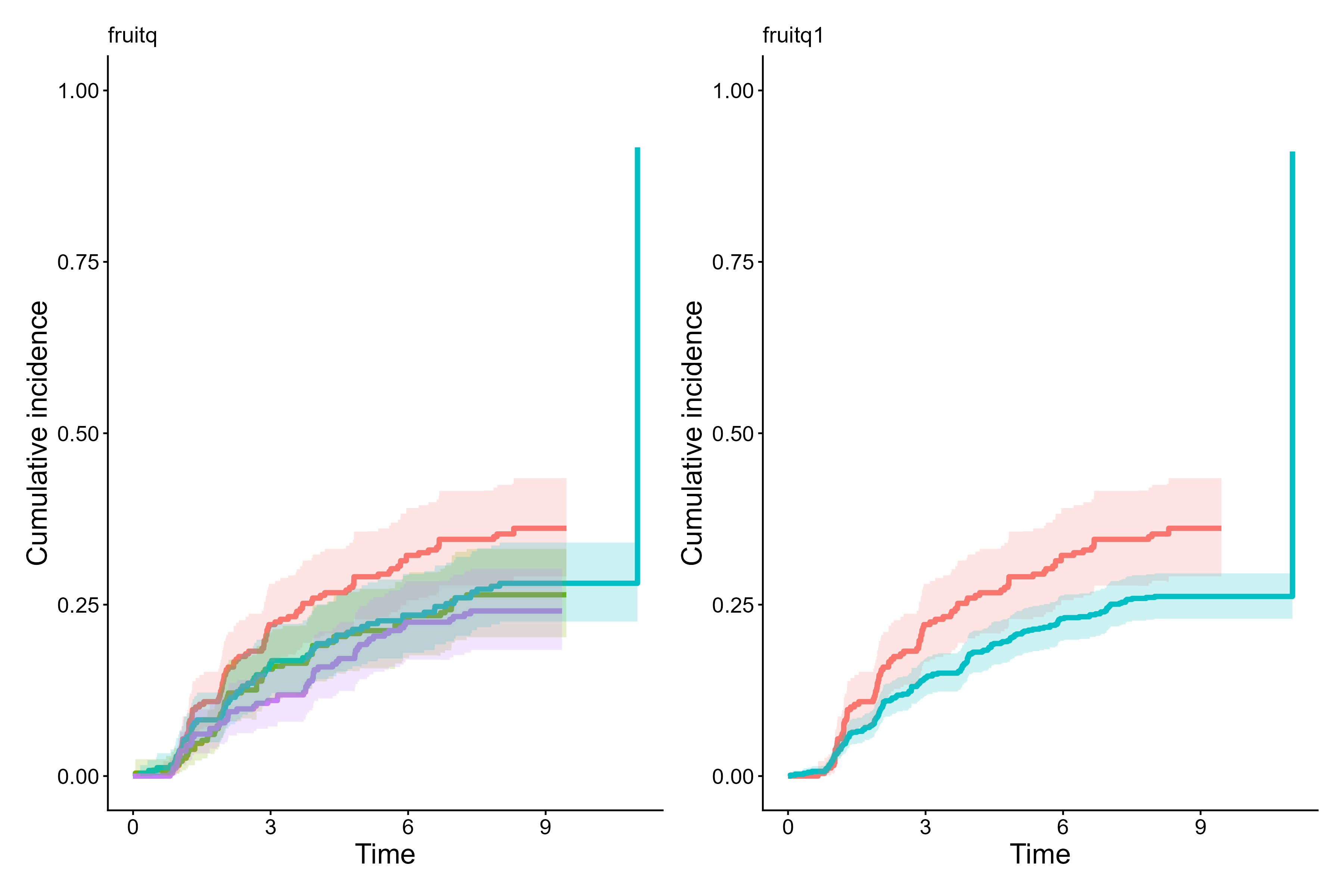
Cumulative incidence curves per each stratification variable
In the second figure, competing-risk marks are added
(add.competing.risk.mark = TRUE) to indicate individuals
who experienced the competing event (macrovascular complications) before
diabetic retinopathy. Here we show a workflow slightly different from
the previous code. First, we compute a survfit-compatible object
output1 using cifcurve() with
outcome.type="competing-risk" by calculating Aalen–Johansen
estimator stratified by fruitq1. The time points at which
the macrovascular complications occurred were obtained as
output2 for each strata using a helper function
extract_time_to_event(). Then, cifplot() is
used to generate the figure. These marks help distinguish between events
due to the primary cause and those attributable to competing causes.
Note that the names of competing.risk.time and
intercurrent.event.time must match the strata labels used
in the plot if supplied by the user. The label.y,
label.x and limit.x arguments are also used to
customize the axis labels and limits.
output1 <- cifcurve(Event(t,epsilon)~fruitq1, data=diabetes.complications,
                    outcome.type="competing-risk")
output2 <- extract_time_to_event(Event(t,epsilon)~fruitq1,
                                 data=diabetes.complications, which.event="event2")
cifplot(output1, add.conf=FALSE, add.risktable=FALSE,
        add.censor.mark=FALSE, add.competing.risk.mark=TRUE, competing.risk.time=output2,
        label.y="CIF of diabetic retinopathy", label.x="Years from registration",
        limits.x=c(0,8))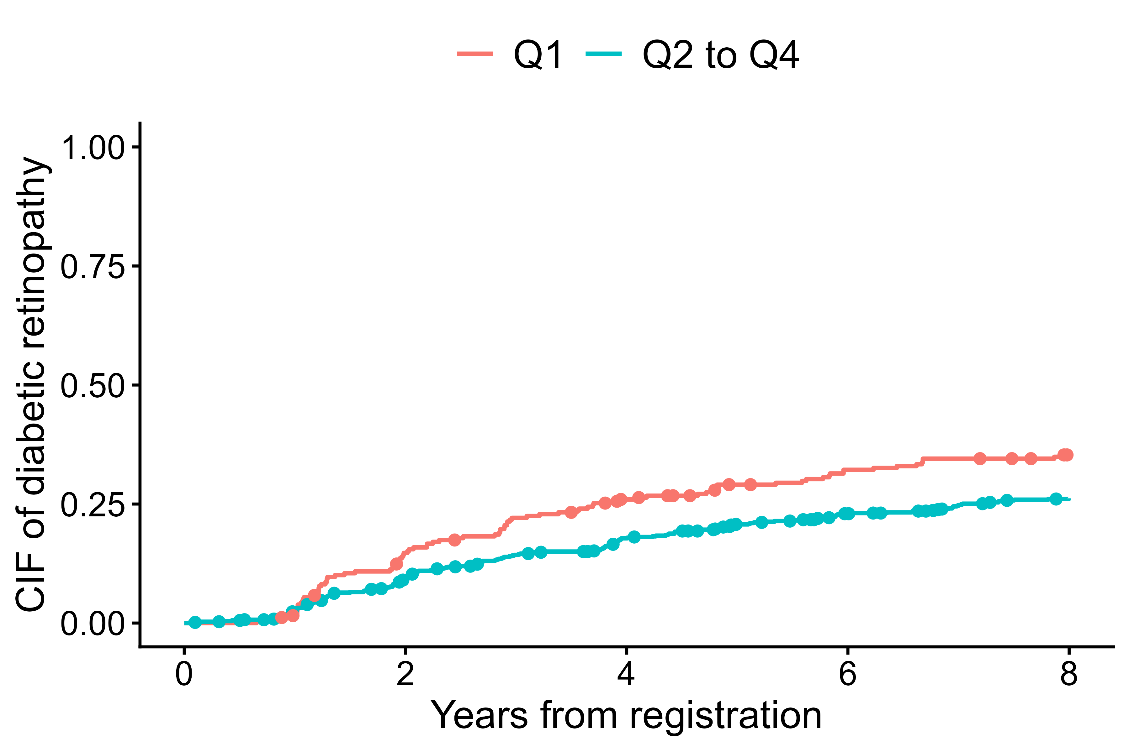
Cumulative incidence curves with competing risk marks
The label.strata is another argument for customizing
labels, but when inputting a survfit object, it becomes invalid because
it does not contain stratum information. Therefore, the following code
inputs the formula and data. label.strata is used by
combining level.strata and order.strata. The
level.strata specifies the levels of the
stratification variable corresponding to each label in
label.strata. The levels specified in
level.strata are then displayed in the figure in
the order defined by order.strata. A figure
enclosed in a square was generated, which is due to
style="framed" specification.
cifplot(Event(t,epsilon)~fruitq1, data=diabetes.complications,
        outcome.type="competing-risk", add.conf=FALSE, add.risktable=FALSE,
        add.estimate.table=TRUE, add.censor.mark=FALSE, add.competing.risk.mark=TRUE,
        competing.risk.time=output2, label.y="CIF of diabetic retinopathy",
        label.x="Years from registration", limits.x=c(0,8),
        label.strata=c("High intake","Low intake"), level.strata=c("Q2 to Q4","Q1"),
        order.strata=c("Q1", "Q2 to Q4"), style="framed")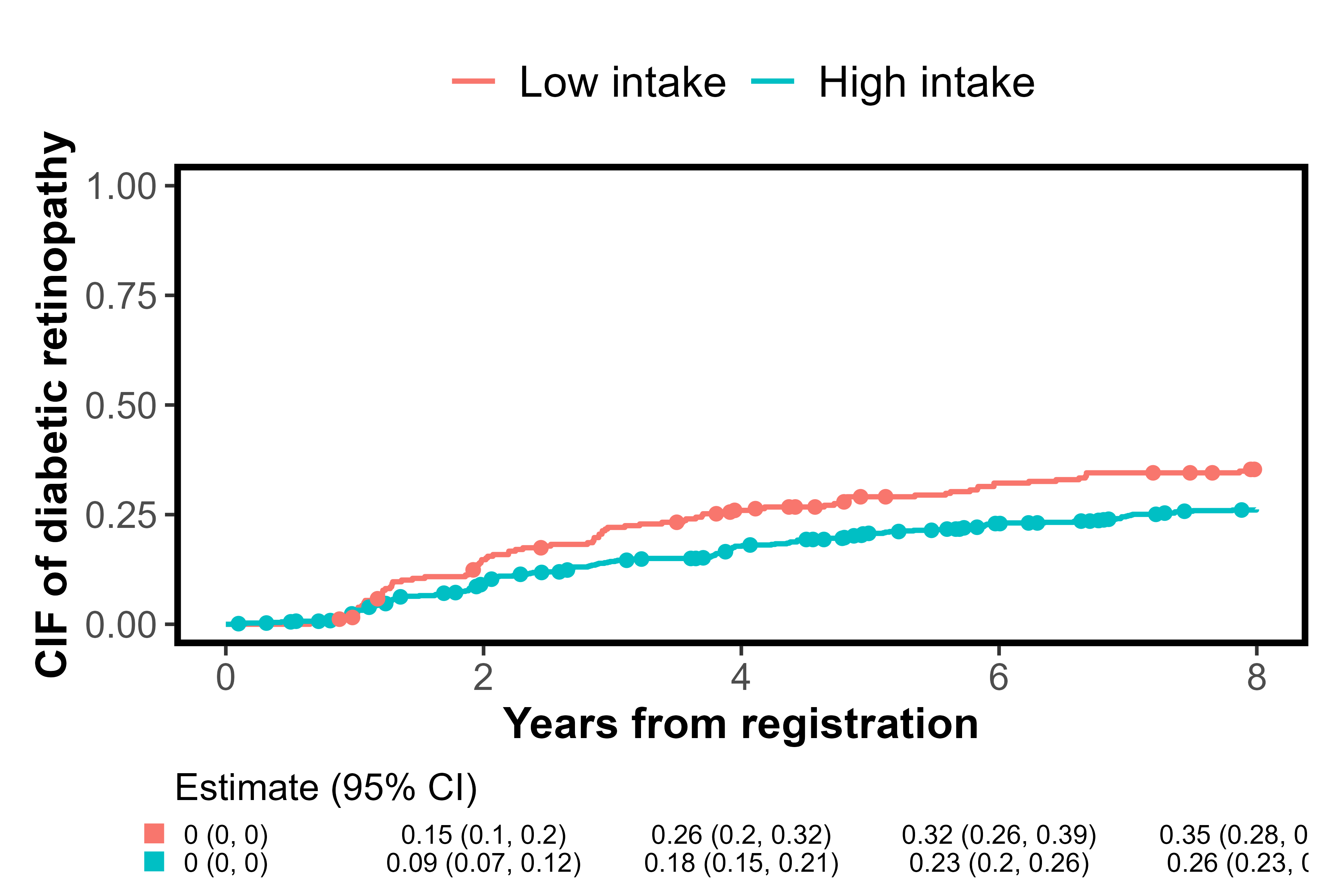
Cumulative incidence curves with strata labels and framed style
By specifying add.estimate.table = TRUE, the
risks of diabetic retinopathy (estimates for CIFs) along with their
CIs are shown in the table at the bottom of the figure. The
risk ratios at a specific time point (e.g. 8 years) for competing events
can be jointly and coherently estimated using polyreg()
with outcome.type = "competing-risk". In the code of
polyreg() below, no covariates are included in the nuisance
model (~1 specifies intercept only). The effect of low
fruit intake fruitq1 is estimated as an unadjusted
risk ratio (effect.measure1="RR") for diabetic
retinopathy (event 1) and macrovascular complications (event 2) at 8
years (time.point=8).
output3 <- polyreg(nuisance.model=Event(t,epsilon)~1, exposure="fruitq1",
          data=diabetes.complications, effect.measure1="RR", effect.measure2="RR",
          time.point=8, outcome.type="competing-risk",
          report.nuisance.parameter=TRUE)
coef(output3)
#> [1] -1.38313159 -0.30043942 -3.99147406 -0.07582595
vcov(output3)
#>              [,1]         [,2]         [,3]         [,4]
#> [1,]  0.017018160 -0.012351309  0.009609321 -0.008372500
#> [2,] -0.012351309  0.012789187 -0.006012254  0.006540183
#> [3,]  0.009609321 -0.006012254  0.048161715 -0.044070501
#> [4,] -0.008372500  0.006540183 -0.044070501  0.055992232
summary(output3)
#>
#>                       event1        event2
#> ----------------------------------------------
#> Intercept
#>                       0.251         0.018
#>                       [0.194, 0.324]  [0.012, 0.028]
#>                       (p=0.000)     (p=0.000)
#>
#> fruitq1, Q2 to Q4 vs Q1
#>                       0.740         0.927
#>                       [0.593, 0.924]  [0.583, 1.474]
#>                       (p=0.008)     (p=0.749)
#>
#> ----------------------------------------------
#>
#> effect.measure        RR at 8       RR at 8
#> n.events              279 in N = 978  79 in N = 978
#> median.follow.up      8             -
#> range.follow.up       [0.05, 11.00]  -
#> n.parameters          4             -
#> converged.by          Converged in objective function  -
#> nleqslv.message       Function criterion near zero  -
The summary() method prints an event-wise table of point
estimates, CIs, and p-values. Internally, a "polyreg"
object also supports the generics API:
-
tidy(): coefficient-level summaries (one row per term and per event), -
glance(): model-level summaries (follow-up, convergence, number of events), -
augment(): observation-level diagnostics (weights for IPCW, predicted CIFs, and influence-functions).
This means that polyreg() fits integrate naturally with
the broader broom/modelsummary ecosystem. For
publication-ready tables, you can pass polyreg objects
directly to modelsummary::msummary(), including
exponentiated summaries (risk ratios, odds ratios, subdistribution
hazard ratios) via the exponentiate = TRUE option.
Example 2. Survival analysis
The second example is time to first event analysis
(outcome.type="survival") to estimate the effect on the
risk of diabetic retinopathy or macrovascular complications at 8 years.
In the code below, cifplot() is directly used to generate a
survfit-compatible object internally and plot it.
diabetes.complications$d <- as.integer(diabetes.complications$epsilon>0)
cifplot(Event(t,d) ~ fruitq1, data=diabetes.complications,
outcome.type="survival", add.conf=TRUE, add.censor.mark=FALSE,
add.competing.risk.mark=FALSE, label.y="Survival (no complications)",
label.x="Years from registration", label.strata=c("High intake","Low intake"),
level.strata=c("Q2 to Q4","Q1"), order.strata=c("Q1", "Q2 to Q4"))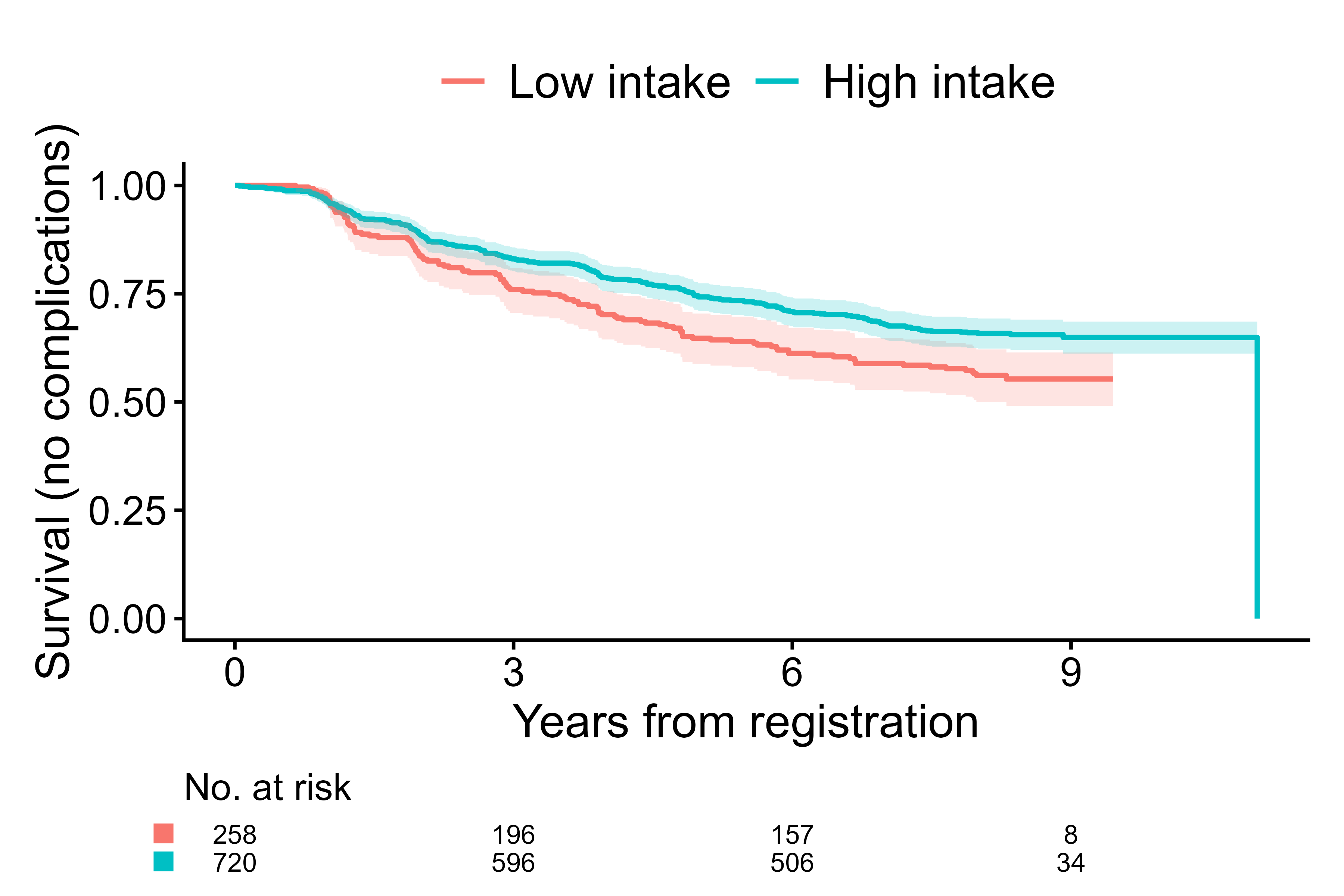
Survival curves from cifplot()
The code below specifies the Richardson model (Richardson, Robins and
Wang 2017) on the risk of diabetic retinopathy or macrovascular
complications at 8 years (outcome.type=“survival”). Dependent censoring
is adjusted by stratified IPCW method (strata='strata').
Estimates other than the effects of exposure (e.g. intercept) are
suppressed when report.nuisance.parameter is not
specified.
output4 <- polyreg(nuisance.model=Event(t,d)~1,
          exposure="fruitq1", strata="strata", data=diabetes.complications,
          effect.measure1="RR", time.point=8, outcome.type="survival")
summary(output4)
#>
#>                       event 1 (no competing risk)
#> ----------------------------------
#> fruitq1, Q2 to Q4 vs Q1
#>                       0.777
#>                       [0.001, 685.697]
#>                       (p=0.942)
#>
#> ----------------------------------
#>
#> effect.measure        RR at 8
#> n.events              358 in N = 978
#> median.follow.up      8
#> range.follow.up       [0.05, 11.00]
#> n.parameters          2
#> converged.by          Converged in objective function
#> nleqslv.message       Function criterion near zero
Example 3. Adjusted competing risks analysis
The code below specifies direct polytomous regression for both of
competing events (outcome.type="competing-risk"). Here 15
covariates and censoring strata are specified in
nuisance.model= and strata=, respectively.
output5 <- polyreg(nuisance.model=Event(t,epsilon)~age+sex+bmi+hba1c
          +diabetes_duration+drug_oha+drug_insulin+sbp+ldl+hdl+tg
          +current_smoker+alcohol_drinker+ltpa,
          exposure="fruitq1", strata="strata", data=diabetes.complications,
          effect.measure1="RR", time.point=8, outcome.type="competing-risk")
summary(output5)
#>
#>                       event1        event2
#> ----------------------------------------------
#> fruitq1, Q2 to Q4 vs Q1
#>                       0.644         1.100
#>                       [0.489, 0.848]  [0.596, 2.030]
#>                       (p=0.002)     (p=0.761)
#>
#> ----------------------------------------------
#>
#> effect.measure        RR at 8       RR at 8
#> n.events              279 in N = 978  79 in N = 978
#> median.follow.up      8             -
#> range.follow.up       [0.05, 11.00]  -
#> n.parameters          32            -
#> converged.by          Converged in objective function  -
#> nleqslv.message       Function criterion near zero  -
Example 4. Description of cumulative incidence of competing events
The cifpanel() arranges multiple survival and CIF plots
into a single, polished layout with a shared legend. It’s designed for
side-by-side comparisons—e.g., event 1 vs event 2, different groupings,
or different y-scales—while keeping axis ranges and styles consistent.
Internally each panel is produced using the same engine as
cifcurve(), and you can supply scalar arguments (applied to
all panels) or lists to control each panel independently.
This function accepts both shared and panel-specific
arguments. When a single formula is provided, the same model
structure is reused for each panel, and arguments supplied as lists are
applied individually to each panel. Arguments such as
code.events, label.strata, or
add.censor.mark can be given as lists, where each list
element corresponds to one panel. This allows flexible configuration
while maintaining a concise and readable syntax.
The example below creates a 1×2 panel
(rows.columns.panel = c(1,2)) comparing the
cumulative incidence of two competing events in the same
cohort, namely CIF of diabetic retinopathy in the left panel
and CIF of macrovascular complications in the right panel. Both panels
are stratified by fruitq1, and the legend is shared at the
bottom. The pairs of code.events as a list instructs
cifpanel() to display event 1 in the first panel and event
2 in the second panel, with event code 0 representing censoring.
output6 <- cifpanel(
 rows.columns.panel = c(1,2),
 formula            = Event(t, epsilon) ~ fruitq1,
 data               = diabetes.complications,
 outcome.type       = "competing-risk",
 code.events        = list(c(1,2,0), c(2,1,0)),
 label.y            = c("CIF of diabetic retinopathy", "CIF of macrovascular complications"),
 label.x            = "Years from registration",
 label.strata       = list(c("High intake","Low intake")),
 title.plot         = c("Diabetic retinopathy", "Macrovascular complications"),
 legend.position    = "bottom",
 legend.collect     = TRUE
)
print(output6)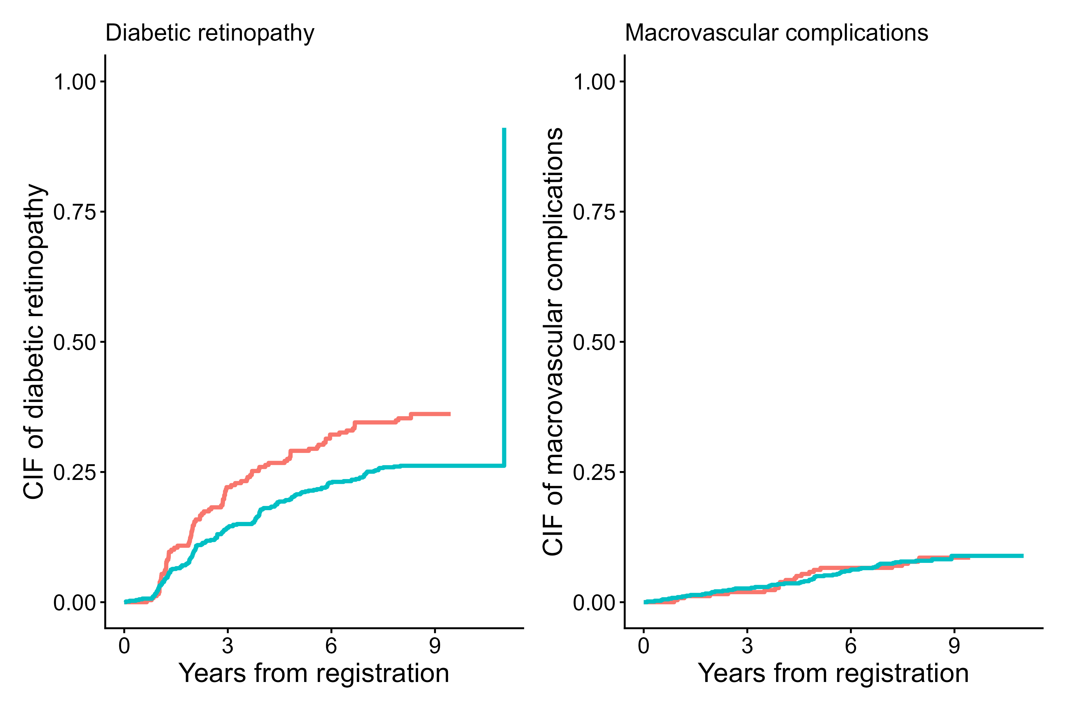
Cumulative incidence curves for event 1 vs event 2 using cifpanel()
Arguments specified as scalars (for example,
label.x = "Years from registration") are applied
uniformly to all panels. Character vectors of the same length
as the number of panels (for example,
label.y = c("Diabetic retinopathy", "Macrovascular complications"))
assign a different label to each panel in order. Lists provide the most
flexibility, allowing each panel to have distinct settings that mirror
the arguments of cifcurve().
The legend.collect = TRUE option merges legends from all
panels into a single shared legend, positioned according to
legend.position. The arguments title.panel,
subtitle.panel, caption.panel, and
title.plot control the overall panel title and individual
subplot titles, ensuring that multi-panel layouts remain consistent and
publication-ready.