generate_data <- function(n = 200, hr1, hr2) {
  # Stoma: 1 = with stoma, 0 = without stoma
  stoma <- rbinom(n, size = 1, prob = 0.4)
  # Sex: 0 = WOMAN, 1 = MAN
  sex <- rbinom(n, size = 1, prob = 0.5)
  # Age: normal distribution (stoma group slightly older)
  age <- rnorm(n, mean = 65 + 3 * stoma, sd = 8)

  # Hazards for relapse and death (larger hazard implies earlier event)
  hazard_relapse   <- ifelse(stoma == 1, hr1 * 0.10, 0.10)
  hazard_death     <- ifelse(stoma == 1, hr2 * 0.10, 0.10)
  hazard_censoring <- 0.05

  # Latent times to relapse, death, and censoring
  t_relapse   <- rexp(n, rate = hazard_relapse)
  t_death     <- rexp(n, rate = hazard_death)
  t_censoring <- rexp(n, rate = hazard_censoring)

  # Overall survival (OS)
  # status_os = 1 → death (event of interest)
  # status_os = 0 → censored
  time_os   <- pmin(t_death, t_censoring)
  status_os <- as.integer(t_death <= t_censoring)  # 1 = death, 0 = censored

  # Relapse-free survival (RFS)
  # status_rfs = 1 → relapse or death whichever comes first (event of interest)
  # status_rfs = 0 → censored
  time_rfs   <- pmin(t_relapse, t_death, t_censoring)
  status_rfs <- integer(n)
  status_rfs[time_rfs == t_relapse & time_rfs < t_censoring] <- 1  # relapse
  status_rfs[time_rfs == t_death   & time_rfs < t_censoring] <- 1  # death

  # Cumulative incidence of relapse (CIR)
  # status_cir = 1 → relapse (event of interest)
  # status_cir = 2 → death as competing risk
  # status_cir = 0 → censored

  time_cir <- pmin(t_relapse, t_death, t_censoring)
  status_cir <- integer(n)
  status_cir[time_cir == t_relapse & time_cir < t_censoring] <- 1
  status_cir[time_cir == t_death   & time_cir < t_censoring] <- 2

  data.frame(
    id         = 1:n,
    sex        = factor(sex, levels = c(0, 1), labels = c("WOMAN", "MAN")),
    age        = age,
    stoma      = factor(stoma, levels = c(0, 1),
                        labels = c("WITHOUT STOMA", "WITH STOMA")),
    time_os    = time_os,
    status_os  = status_os,
    time_rfs   = time_rfs,
    status_rfs = status_rfs,
    time_cir   = time_cir,
    status_cir = status_cir
  )
}P-Value Explanations That Seem Plausible at First Glance
What is the true meaning of p-values in clinical trials? A coffee-chat guide to confirm the concept of hypothetical repetitions—the frequentist approach—through conversation. This piece cultivates an intuitive understanding of p-values.

Frequentist Thinking II − P-Value Explanations That Seem Plausible at First Glance
Keywords: clinical trial, language & writing, p-value, survival & competing risks
Survival curves and hazard ratios
Daughter: “Dad, I’ve made another cup of coffee. Can you keep going and explain the hazard ratios from JCOG9502?”
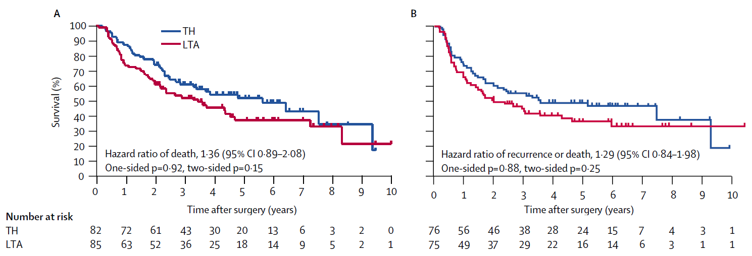
Dad: “Ouch, it’s hot. You’re referring to the hazard ratio of death of 1.36 in Figure A, and the hazard ratio of recurrence or death of 1.29 in Figure B. Both summarize the treatment contrast on the hazard scale, which in turn drives the separation you see in the Kaplan-Meier curves, showing that the TH group had better outcomes than the LTA group. A higher hazard means the Kaplan-Meier curve tends to drop more quickly. What matters here is that both overall survival (OS) in Figure A and disease-free survival (DFS) in Figure B have shapes that are well summarized by a hazard ratio.”
Daughter: “Summarized well—meaning what, exactly?”
Dad: “Yes. In both figures, the Kaplan-Meier curve for the TH group lies cleanly above that for the LTA group—except at the far right, where only four patients remain and the curves cross. The hazard ratio assumes that the two survival curves are proportional on the hazard scale. Although it’s not explicitly stated in the figures, the hazard ratios are reported so that values above 1 correspond to worse outcomes in the LTA group relative to TH. This relationship is what we call Cox regression or the proportional hazards model.”
Daughter: “So if the curves cross, that breaks the proportional hazards assumption.”
Dad: “Exactly. And the OS and DFS results are consistent with each other as well. That makes the findings very straightforward and easy to interpret. I’ll show you Cox regression in R later.”
Daughter: “Thanks—later then. But looking at these figures, the hazard ratios are 1.36 and 1.29, right? A higher hazard means the Kaplan-Meier curve drops faster, and the reference is the TH group. So if the hazard ratio is greater than one, the LTA group did worse than the TH group in OS and DFS. And p-values below 0.05 are considered statistically significant, right? So the LTA group had worse outcomes, but since the p-values aren’t below the threshold, there’s no statistically significant difference between the two groups?”
Dad: “That’s right. The hazard reflects the speed at which death or recurrence occurs, and the hazard ratio is simply the ratio between the two groups.”
P-value explanations that seem plausible
Dad: “The precise meaning of p-values is often misunderstood. One thing to keep in mind when reading papers is that the threshold compared against the p-value—the significance level—may not always be 5%. For example, consider interim analyses. Take a look at the abstract. In JCOG9502, an interim analysis was planned before the final analysis, and this paper reports results after the trial was stopped early. In interim analyses, it’s common to test using a significance level lower than 5%.”
Daughter: “So the trial was stopped early because it became statistically significant?”
Dad: “No. The trial was stopped not because a significant difference was found, but because the data and safety monitoring committee judged that there was no reasonable chance that the LTA group would prove superior. There are several other common misunderstandings. Look at these statements.”
A p-value is the probability that the null hypothesis is true.
A small p-value and statistical significance mean that an important scientific finding has been obtained.
A statistically non-significant result means that the null hypothesis is true and should be accepted.
Dad: “In JCOG9502, the null hypothesis is that the overall survival curves of the LTA and TH groups are equal. Let me ask you about the first statement. Do you think the p-value in JCOG9502 represents the probability that ‘there is no difference between the survival curves of the LTA and TH groups’?”
Daughter: “This is starting to feel like a blackboard lecture. Was mentioning statistics textbooks a mistake? But sure—statement one sounds fine to me. If the p-value is 0.05, then it’s correct five times out of a hundred, right?”
Dad: “Here I want you to choose your words carefully. Is the statement ‘there is no difference between the survival curves’ a random variable? It isn’t. A proposition is either true or false. Defining a probability for something that is not a random variable is conceptually problematic.”
Daughter: “Ah, that’s the distinction you wanted me to notice. Fine—I’ll stop phrasing it that way.”
Dad: “Then what did you mean by ‘five times out of a hundred’?”
Daughter: “Literally that. If we ran JCOG9502 a hundred times, what would happen?”
Dad: “Exactly. If you repeat the same trial a hundred times, you get a hundred p-values. That’s the definition of probability in this context—frequentist probability. Now let’s move on. Do you think a small p-value means that an important scientific discovery has been made?”
Daughter: “Isn’t that how people usually think about it?”
Dad: “But look at the p-values shown in the figure—four of them, ranging from 0.15 to 0.92. None are small. Does that mean the results aren’t scientifically important?”
Daughter: “No, that’s not what I meant.”
Dad: “Exactly. The idea that smaller p-values imply more important scientific findings is simply wrong. If you focus too much on p-values, your interpretation of a paper can easily become distorted.”
Daughter: “Okay, okay. But aren’t you talking a bit too long?”
Dad: “Let’s consider the third statement: ‘A statistically non-significant result means that the null hypothesis is true and should be accepted.’ Is that correct?”
Daughter: “I remember reading that p-values are used to reject hypotheses, not to accept them. So this must be wrong too. But in practice, what happens when a result isn’t significant? If a clinical trial compares drug A and drug B, can we conclude that they’re equivalent?”
Dad: “That would be breaking the rules. If the null hypothesis were true, it would mean that A and B are equivalent—but you cannot accept it just because there’s no significant difference. To conclude equivalence or non-inferiority, you need a properly designed equivalence trial or non-inferiority trial.”
Daughter: “Right. I suspected that, but it helps to hear it stated clearly.”
Dad: “This distinction had to be built into the rules, and history shows why. About thirty years ago in Japan, non-inferiority trials were required for drug approval. Based on that experience, the relationship between research hypotheses and statistical decision rules has to be handled very carefully.”
NoteCommon misreadings
A p-value is not the probability that the null hypothesis is true. A small p-value does not automatically mean that the result is scientifically or clinically important. A large p-value does not mean “there is no difference,” “the treatments are equivalent,” or “the study has no value.”
When reading a p-value, check at least the null hypothesis, outcome, significance level, test, interim analyses, and multiplicity rules in the Methods. A p-value is not a standalone number; it gets its meaning from the study design and analysis rule.
P-values as a standardized rule
Daughter: “I understand the textbook explanation, but I still feel a gap between theory and reality. About statement two—the idea that ‘small p-values mean important science.’ In basic research, results without significance often get dismissed. That’s the reality. But JCOG9502 is different. It didn’t show superiority of LTA, nor equivalence of the procedures—yet it was published in Lancet Oncology. Why?”
Dad: “I don’t think a negative clinical trial lacks value. Clinical trials are primarily evaluations of technical performance—of surgeries or drugs. Whether efficacy is demonstrated or not, the evaluation itself still has value.”
Daughter: “So even a negative trial has the same informational value?”
Dad: “Yes—if it’s well designed and well executed. Think of a clinical trial as an exam. Passing or failing doesn’t change the value of the score itself. The p-value functions like a grading rule or a technical standard—it’s unavoidable. …Though of course, scores aren’t everything.”
Daughter: “So clinical trials are about evaluating technology, not making scientific discoveries?”
Dad: “Historically, clinical trials developed within regulatory systems for technology evaluation. Standardizing p-values and efficacy endpoints was part of maintaining consistent testing standards. In the 1990s, regulatory requirements still differed across countries. In the late 1990s, regulators in the US, Europe, and Japan agreed on common standards—the ICH guidelines.”
Daughter: “But that’s for industry-sponsored trials, not investigator-initiated studies. And haven’t clinical trials driven paradigm shifts? Cytotoxic drugs, anti-PD-1 antibodies, ADCs. Calling all that ‘technology evaluation’ feels unsatisfying.”
Dad: “Perhaps technology evaluation stimulated science.”
Daughter: “You really like separating technology and science. I’m fine with classifying industry trials as technology evaluation. But in the broader scientific enterprise, clinical trials generate new hypotheses and new questions. That’s what I want to call science.”
NoteA cautionary tale: Hopate
This story is a Japan-specific regulatory episode, but the lesson is general. It’s a cautionary tale about treating ‘no statistically significant difference’ as evidence of equivalence.
Have you heard of the older drug called cerebral circulation and metabolism enhancing agents? This medication was once used for cerebrovascular disorders and dementia, and reportedly generated cumulative sales of around 800 billion yen in Japan. Several similar drugs existed, but most were approved based on “non-inferiority trials” comparing them to the first-approved drug, calcium hopantenate (brand name Hopate). However, the studies conducted at the time did not perform formal non-inferiority analyses setting a non-inferiority margin; instead, non-inferiority was determined based on the finding that there was “no significant difference compared to calcium hopantenate.” Calcium hopantenate was withdrawn from the market in 1989 due to side effects. Around the same time, the Ministry of Health and Welfare (as it was then) requested pharmaceutical companies to conduct reevaluations using placebo-controlled trials. The results showed that none of the cerebral circulation-improving drugs outperformed placebo (Ministry of Health and Welfare, Pharmaceutical Safety Bureau, 1998). This tragedy clearly demonstrates that concluding equivalence or non-inferiority when no significant difference is found is a mistake.
NoteEstimation of a hazard ratio using coxph()
There are several methods for estimating hazard ratios, but the most popular is the coxph() function in the survival package. In a previous episode, we used the function generate_data(hr1, hr2) to generate data on the presence of a stoma and overall survival (OS). This time, we will apply Cox regression to the same data and calculate the hazard ratio between the stoma group and the non-stoma group. In generate_data(hr1, hr2), the true value of the hazard ratio for death can be specified using the hr2 argument.
NoteR code for generate_data()
NoteR code for coxph() and outout
#- Generation of data frame "dat" --------------------------
dat <- generate_data(hr1 = 2, hr2 = 1.5)  # true HR for death = 1.5

#- Analysis using coxph() ----------------------------------
# install.packages("survival") # if needed
library(survival)

fit <- coxph(Surv(time_os, status_os) ~ stoma, data = dat)
summary(fit)
Call:
coxph(formula = Surv(time_os, status_os) ~ stoma, data = dat)
n= 200, number of events= 140
coef exp(coef) se(coef) z Pr(>|z|)
stomaWITH STOMA 0.4227 1.5261 0.1726 2.449 0.0143 *
---
Signif. codes: 0 '***' 0.001 '**' 0.01 '*' 0.05 '.' 0.1 ' ' 1
exp(coef) exp(-coef) lower .95 upper .95
stomaWITH STOMA 1.526 0.6553 1.088 2.14
Concordance= 0.556 (se = 0.024 )
Likelihood ratio test= 5.93 on 1 df, p=0.01
Wald test = 6 on 1 df, p=0.01
Score (logrank) test = 6.08 on 1 df, p=0.01Reference
Sasako M, Sano T, Yamamoto S, Sairenji M, Arai K, Kinoshita T, Nashimoto A, Hiratsuka M, Japan Clinical Oncology Group (JCOG9502). Left thoracoabdominal approach versus abdominal-transhiatal approach for gastric cancer of the cardia or subcardia: a randomised controlled trial. Lancet Oncol 2006;7(8):644-51
Next episode and R script
NoteOther episodes
Episodes in this series
- Reading a Paper over a Cup of Coffee
- P-Value Explanations That Seem Plausible at First Glance
- Beyond 0.05: Interpreting P-Values in a Clinical Trial
Earlier series
Glossary