generate_data <- function(n = 200, hr1, hr2, hr3) {
  stoma <- rbinom(n, size = 1, prob = 0.4)
  sex <- rbinom(n, size = 1, prob = 0.5)
  age <- rnorm(n, mean = 65 + 3 * stoma, sd = 8)
  hazard_relapse   <- 0.10*exp(stoma*log(hr1)+age*log(hr2))
  hazard_death     <- ifelse(stoma == 1, hr3 * 0.10, 0.10)
  hazard_censoring <- 0.05

  t_relapse   <- rexp(n, rate = hazard_relapse)
  t_death     <- rexp(n, rate = hazard_death)
  t_censoring <- rexp(n, rate = hazard_censoring)

  time_os   <- pmin(t_death, t_censoring)
  status_os <- as.integer(t_death <= t_censoring)

  time_rfs <- pmin(t_relapse, t_death, t_censoring)
  status_rfs <- integer(n)
  status_rfs[time_rfs == t_relapse & time_rfs < t_censoring] <- 1
  status_rfs[time_rfs == t_death & time_rfs < t_censoring] <- 1

  time_cir <- pmin(t_relapse, t_death, t_censoring)
  status_cir <- integer(n)
  status_cir[time_cir == t_relapse & time_cir < t_censoring] <- 1
  status_cir[time_cir == t_death & time_cir < t_censoring] <- 2

  dat <- data.frame(
    id         = 1:n,
    sex        = factor(sex, levels = c(0, 1), labels = c("WOMAN", "MAN")),
    age        = age,
    stoma      = factor(stoma, levels = c(0, 1),
                        labels = c("WITHOUT STOMA", "WITH STOMA")),
    time_os    = time_os,
    status_os  = status_os,
    time_rfs   = time_rfs,
    status_rfs = status_rfs,
    time_cir   = time_cir,
    status_cir = status_cir
  )
}From Risk and Rate to Survival and Hazard
A coffee-chat guide to the basics of survival analysis. We connect risk, survival curves, rates, hazards, and hazard ratios, and use simple simulation code to make the time dimension visible.

Effects and Time IV − From Risk and Rate to Survival and Hazard
Keywords: effect measure, probability model, R simulation, survival & competing risks
Risk and time
Me: “Dad, I was thinking back to the attributable fraction discussion. Something still doesn’t quite sit right.”
Dad: “That sounds like a good reason for coffee.”
Me: “You said the attributable fraction can change when we look 10, 12, or 20 years after screening. That means risk has time hidden inside it. Isn’t that no longer binary data? Isn’t it survival-time data?”
Dad: “Exactly. Risk and survival curves are two sides of the same coin.”
Me: “So if I read a survival probability from a survival curve at a certain time point, one minus that is the risk by that time. And the epidemiologic idea of a rate connects to the survival-analysis idea of a hazard. What still bothers me is the hazard ratio. Risk ratios can change over time, but is a hazard ratio supposed to stay constant?”
Dad: “In Cox regression, we often assume it is constant over time. More precisely, even if the survival curves themselves are changing, the model forces the ratio of the hazards to be constant.”
Me: “The risk ratio changes but the hazard ratio doesn’t? That sounds contradictory.”
Dad: “It feels that way because risk is accumulated over time from the hazard. Let’s start with risk and hazard.”
NoteSurvival curves and hazards
In earlier episodes, we discussed risk by a fixed time point. Now we move to Kaplan-Meier curves, which estimate risk as it changes over time.
A Kaplan-Meier curve is an estimate from survival-time data plotted against time. In mathematical notation, we can write the survival curve as a function of time, \(S(x)\).
To see the relationship between survival and hazard, consider a very simple case where the hazard is constant over time. That corresponds to an exponential distribution. If the hazard is denoted by \(\lambda\), the survival function is:
\[ S(x)=\mathrm{exp}(-\lambda x) \]
The disease risk by time \(x\), denoted by \(\pi\), is:
\[ \pi=1-S(x)=1-\mathrm{exp}(-\lambda x) \]
So risk and hazard are connected through time. A risk is not just a static number; it is a probability accumulated up to a particular time point.
Me: “I am not fluent in equations.”
Dad: “Fair. The important point is what the equation connects. With an exponential distribution, the hazard is treated as a constant, while the survival function changes over time. A simulation can make that easier to see.”
NoteCode for generate_data()
NoteKaplan-Meier curves with cifplot()
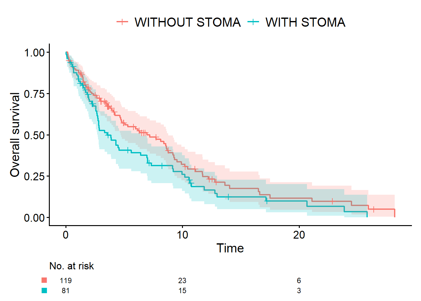
To make the simulated data easier to see, here is a Kaplan-Meier curve drawn with cifplot(), together with a Cox regression fit.
NoteR code for cifplot()
# devtools::install_github("gestimation/cifmodeling") # if needed
library(cifmodeling)
set.seed(46)
dat <- generate_data(hr1=2, hr2=1, hr3=1.5)
cifplot(Event(time_os, status_os) ~ stoma,
  data         = dat,
  outcome.type = "survival",
  label.y      = "Overall survival"
)
NoteR code for coxph()
# install.packages("survival") # if needed
library(survival)
fit <- coxph(Surv(time_os, status_os) ~ stoma, data = dat)
summary(fit)
Call:
coxph(formula = Surv(time_os, status_os) ~ stoma, data = dat)
n= 200, number of events= 144
coef exp(coef) se(coef) z Pr(>|z|)
stomaWITH STOMA 0.3199 1.3769 0.1693 1.889 0.0589 .
---
Signif. codes: 0 '***' 0.001 '**' 0.01 '*' 0.05 '.' 0.1 ' ' 1
exp(coef) exp(-coef) lower .95 upper .95
stomaWITH STOMA 1.377 0.7262 0.9881 1.919
Concordance= 0.544 (se = 0.024 )
Likelihood ratio test= 3.51 on 1 df, p=0.06
Wald test = 3.57 on 1 df, p=0.06
Score (logrank) test = 3.6 on 1 df, p=0.06Me: “So specifying a hazard under an exponential distribution determines the survival curve.”
Dad: “Right. The hazard itself is hard to picture, so it often helps to connect it with median survival. The median is the time when the survival curve reaches 50%.”
NoteHazard and median survival time
The hazard controls how quickly the survival curve falls. If median survival time is denoted by \(M\), then under an exponential distribution:
\[ 0.5=\mathrm{exp}(-\lambda M) \]
Therefore:
\[ M = \frac{\log 2}{\lambda} \approx \frac{0.7}{\lambda} \]
Under this simple model, median survival time and the hazard move in opposite directions. If the median survival time doubles, the hazard is cut roughly in half.
Me: “That part I can feel. Hazard is inversely related to lifespan, at least in this simple setting.”
Dad: “Exactly. A hazard ratio compares hazards between two groups:”
\[ HR=\frac{\lambda_1}{\lambda_2} \]
NoteA quiz related to this episode
When is it appropriate to report median survival time?
- When the sample size is at least 100
- When all participants complete planned follow-up
- When at least half of participants have experienced the event
- All of the above are wrong
NoteAnswer
- The correct answer is 3.
Median survival time is the time at which survival probability reaches 50%. If fewer than half of participants have experienced the event, the survival curve has not reached 50%, so the median survival time is not yet estimable.
Next episodes and R script
NoteOther episodes
Episodes in this series
- Silent Confusions Hidden in Percentages
- Who Is This Percentage About? Target Populations and Attributable Fractions
- When Odds Ratios Approximate Risk Ratios—and When They Fail
- From Risk and Rate to Survival and Hazard
- A First Note on Cox Regression
- After Cox Regression: A Case Study and R Demonstration
Earlier series
Glossary