library(survival)
library(cifmodeling)

survfit(Surv(time, status) ~ stoma,
  data         = dat
)
cifplot(Surv(time, status) ~ stoma,
  data         = dat,
  outcome.type = "survival",
  label.y      = "Overall survival"
)
cifplot(Event(time, status) ~ stoma,
  data         = dat,
  outcome.type = "survival",
  label.y      = "Overall survival"
)A First Step into Survival and Competing Risks Analysis with R
In survival analysis, pitfalls often begin with event definitions and coding. A coffee-chat guide covering data collection and a gentle demonstration of competing risks analysis in R. Designed for readers new to time-to-event data.

Study Design IV − A First Step into Survival and Competing Risks Analysis with R
Keywords: bias, R simulation, study design, survival & competing risks
Survey items and types of data
Me: “Oh wow, that takes me back. Is that the Rubik’s Cube I bought when I was in elementary school? You’re still playing with it? If you’ve got a minute, can I ask you something? Remember the study we talked about on return-to-work among cancer survivors? I’ve drafted a questionnaire to send to patients. Could you have a look? Oh, and the R code you showed me last time really helped—I could kind of picture what the results might look like.”
Dad: “Let’s see.”
Table 1. My original questionnaire
| Item | Response |
|---|---|
| Survey date | ____ Year ____ Month ____ Day |
| Surgery date | ____ Year ____ Month ____ Day |
| Were you employed before surgery? | Yes ____ / No ____ |
| For those who were employed: Did you resign because of the surgery? | Yes ____ / No ____ |
| For those who resigned: Did you wish to return to work? | Yes ____ / No ____ |
| For those who wished to return: Were you able to return to work? | Yes ____ / No ____ |
Dad: “How are you defining the return-to-work proportion?”
Me: “What do you mean?”
Dad: “Just from the questionnaire, I can’t tell whether these questions are enough. Are you trying to find out, between the date of surgery and the date of the survey, whether patients who wanted to return to work actually managed to do so?”
Me: “That would be good to know, but among the patients who answer that they don’t want to return, there might be some who gave up because of company policy or other reasons. So when I calculate the return-to-work proportion, I don’t want the denominator to be ‘patients who wished to return to work.’ I’d rather use all patients who had surgery. That feels closer to the real employment situation.”
Dad: “And do you want to look at whether they returned to work between surgery and the survey date?”
Me: “Hmm. The timing of the responses will vary from patient to patient, so I’d rather not use the survey date. How about defining it as ‘return-to-work within 1 year’? Oh—maybe we should also ask them to write down the actual date they returned to work.”
Dad: “Having the date of return-to-work is a good idea. Then, when you turn return-to-work status into analytic ‘variables’, you can think in terms of two options: categorical data and survival data. Setting that aside for a moment—what will you do if a patient dies after surgery?”
Me: “If they die during the hospital stay, I won’t include them in the study population. But it feels strange to exclude deaths from postoperative recurrence from the denominator.”
Dad: “I agree. Excluding them would introduce bias, because you’d be drifting away from your target population. When you follow cancer patients over time, there are three important points. First, you have to decide what the time origin is. In this case, it would be natural to set the time origin at the date of discharge. Second, you set a target follow-up period and try to collect information as completely as possible up to that point. Missing information becomes a source of bias. Third, you must not exclude events that occur after the time origin.”
- Define the time origin.
- Set a target follow-up period and, up to that point, collect information as completely as possible.
- Do not exclude events that occur after the time origin or use them as strata.
Me: “Right, I don’t want to discover later that we built bias into the design. Got it.”
Dad: “Earlier I suggested using the ‘PECO’ elements to structure your clinical question. If P is ‘patients with rectal cancer after curative resection’, then you have to survey that population comprehensively.”
Me: “So what exactly are categorical data and survival data?”
Dad: “We talked about this the other day too. For statistical analysis, the starting point is always the ‘type of data.’ Categorical data and survival data are two examples of data types.”
Me: “That was last week, and I’ve been busy, you know.”
Dad: “I made a few tweaks to your questionnaire, so I’ll use this version to explain it again.”
Table 2A. Questionnaire for survivors
| Item | Response |
|---|---|
| Survey date | ____ Year ____ Month ____ Day |
| Surgery date | ____ Year ____ Month ____ Day |
| Discharge date | ____ Year ____ Month ____ Day |
| Date of return-to-work (post-discharge; only if employed before surgery) | ____ Year ____ Month ____ Day |
| Were you employed before surgery? | Yes ____ / No ____ |
| For those who were employed: Did you resign because of the surgery? | Yes ____ / No ____ |
| For those who resigned: Did you wish to return to work? | Yes ____ / No ____ |
| For those who wished to return: Were you able to return to work? | Yes ____ / No ____ |
Table 2B. Questionnaire for deceased patients
| Item | Response |
|---|---|
| Survey date | ____ Year ____ Month ____ Day |
| Surgery date | ____ Year ____ Month ____ Day |
| Date of death | ____ Year ____ Month ____ Day |
| Were they employed before surgery? | Yes ____ / No ____ |
| Did they return to work after surgery? | Yes ____ / No ____ |
*Enter data from medical records
Dad: “In this setting, categorical data means that you classify patients according to their outcome. You were thinking of using ‘returning to work within 1 year’ as the outcome, right?”
Me: “Yes.”
Dad: “For example, if you label ‘returned within 1 year’ as category 1 and ‘did not return within 1 year’ as category 2, that gives you a type of categorical data called binary data. You can derive it from the questionnaire, and you can calculate the return-to-work proportion.”
Me: “Right. As long as we treat deaths within 1 year as ‘no return to work’.”
Dad: “But when you summarize work status, it’s better not to stick with just two categories. A three-category variable would be more informative. For example:”
- category 1: returned within 1 year
- category 2: did not return within 1 year (for reasons other than death)
- category 3: did not return within 1 year (because of death)
Dad: “That gives you a more detailed picture of the outcomes.”
Me: “Yes, that makes sense. And survival data was…OS, right?”
Dad: “Overall survival (OS) is indeed one kind of survival data. The name is a bit misleading, though—there are many other types. In general, survival data are variables that represent the time from the time origin until an ‘event’.”
Me: “So return-to-work status can also be treated as survival data?”
Dad: “It can. In this case, discharge is a practical time origin. For OS or DFS in clinical trials, surgery or registration is more common. For example, if a patient is discharged on April 1 and returns to work on April 30, the survival time is 29 days (or 30 days if you count both endpoints). Written just as a number of days, it doesn’t look any different from ordinary continuous data, but the essence of survival data is the presence of censoring. If a patient has not returned to work by the survey date, there simply is no actual interval from discharge to return to work.”
Me: “True, but isn’t that fine as it is?”
Dad: “When you use statistical software, you need to add one more piece of information: at the time of the survey, the patient had not yet returned to work—that is, follow-up for return-to-work was censored. That is why survival data always come as a pair of variables.”
A time variable
An event variable
Dad: “For typical survival data, the event variable is binary and indicates whether the event was observed or censored. The time variable, in this case, would be either ‘time from discharge to return-to-work’ or ‘time from discharge to the survey date’.”
NoteEntering survival data
Because survival data consist of a pair of variables, you also need to specify them as a pair when you pass them to R functions. The survival package provides a dedicated input function Surv() for this purpose, which is used by functions such as survfit() and coxph(). The exact input format depends on the package. For example, the mets package defines a separate Event() function. The cifplot() function in the cifmodeling package accepts both Surv() and Event().
Me: “So if the event variable is binary, that means every patient is in exactly 1 of 2 states: either they returned to work or they were censored. Where do deaths go?”
Dad: “If you treat it the way I just described, patients who die are grouped under ‘censored’. But there is another way to handle it, called competing risks. Put simply, a competing risk is an event that prevents the event of interest (such as return-to-work) from being observed.”
Me: “Ah, so in that sense death is a competing risk.”
Dad: “Exactly. Survival data are also called ‘time-to-event data’ in English. Events that occur over time aren’t limited to survival and death. Competing risk models were developed to analyze situations like this. In that case, the event variable becomes a three-category variable: event, competing risk, or censoring. The coding looks like this:”
Event variable = 0: censored before the event is observed
Event variable = 1: event observed
Event variable = 2: competing risk occurs before the event is observed
Me: “I think I get it. I’m going to use this revised questionnaire, then.”
Dad: “Let’s test the idea with a small simulation in R—just enough to see why competing risks matter.”
Survival Analysis and Competing Risk Analysis
NoteGenerating simulation data (with relapse)
Let us now move a little closer to a real clinical research in cancer and compare three outcomes in simulated data: overall survival (OS), relapse-free survival (RFS), and cumulative incidence of relapse (CIR). For CIR, some patients die before recurrence, and we have to decide how to treat those deaths. This is what we call a competing risk.
The code below defines a function, generate_data(), that generates three different survival outcomes in R, including both death and relapse. The event for OS is “death”, and the event for RFS is “death or relapse”. For CIR, the event is “relapse”, and death is treated as a competing risk. We will reuse generate_data() and the resulting simulated data in later explanations.
Stoma: binary data generated from a binomial distribution (
rbinom)Survival time: data generated from an exponential distribution (
rexp) (computed from the random variables t_relapse, t_death, and t_censoring)
In the previous episode, we summarized survival data without competing risks using the Kaplan-Meier curves. In contrast, for competing risks analysis, the appropriate method is not the Kaplan-Meier curves but the Aalen-Johansen curves.
NoteR code for generate_data()
generate_data <- function(n = 200, hr1, hr2) {
  # Stoma: 1 = with stoma, 0 = without stoma
  stoma <- rbinom(n, size = 1, prob = 0.4)
  # Sex: 0 = WOMAN, 1 = MAN
  sex <- rbinom(n, size = 1, prob = 0.5)
  # Age: normal distribution (stoma group slightly older)
  age <- rnorm(n, mean = 65 + 3 * stoma, sd = 8)

  # Hazards for relapse and death (larger hazard implies earlier event)
  hazard_relapse   <- ifelse(stoma == 1, hr1 * 0.10, 0.10)
  hazard_death     <- ifelse(stoma == 1, hr2 * 0.10, 0.10)
  hazard_censoring <- 0.05

  # Latent times to relapse, death, and censoring
  t_relapse   <- rexp(n, rate = hazard_relapse)
  t_death     <- rexp(n, rate = hazard_death)
  t_censoring <- rexp(n, rate = hazard_censoring)

  # Overall survival (OS)
  # status_os = 1 → death (event of interest)
  # status_os = 0 → censored
  time_os   <- pmin(t_death, t_censoring)
  status_os <- as.integer(t_death <= t_censoring)  # 1 = death, 0 = censored

  # Relapse-free survival (RFS)
  # status_rfs = 1 → relapse or death whichever comes first (event of interest)
  # status_rfs = 0 → censored
  time_rfs   <- pmin(t_relapse, t_death, t_censoring)
  status_rfs <- integer(n)
  status_rfs[time_rfs == t_relapse & time_rfs < t_censoring] <- 1  # relapse
  status_rfs[time_rfs == t_death   & time_rfs < t_censoring] <- 1  # death

  # Cumulative incidence of relapse (CIR)
  # status_cir = 1 → relapse (event of interest)
  # status_cir = 2 → death as competing risk
  # status_cir = 0 → censored

  time_cir <- pmin(t_relapse, t_death, t_censoring)
  status_cir <- integer(n)
  status_cir[time_cir == t_relapse & time_cir < t_censoring] <- 1
  status_cir[time_cir == t_death   & time_cir < t_censoring] <- 2

  data.frame(
    id         = 1:n,
    sex        = factor(sex, levels = c(0, 1), labels = c("WOMAN", "MAN")),
    age        = age,
    stoma      = factor(stoma, levels = c(0, 1),
                        labels = c("WITHOUT STOMA", "WITH STOMA")),
    time_os    = time_os,
    status_os  = status_os,
    time_rfs   = time_rfs,
    status_rfs = status_rfs,
    time_cir   = time_cir,
    status_cir = status_cir
  )
}
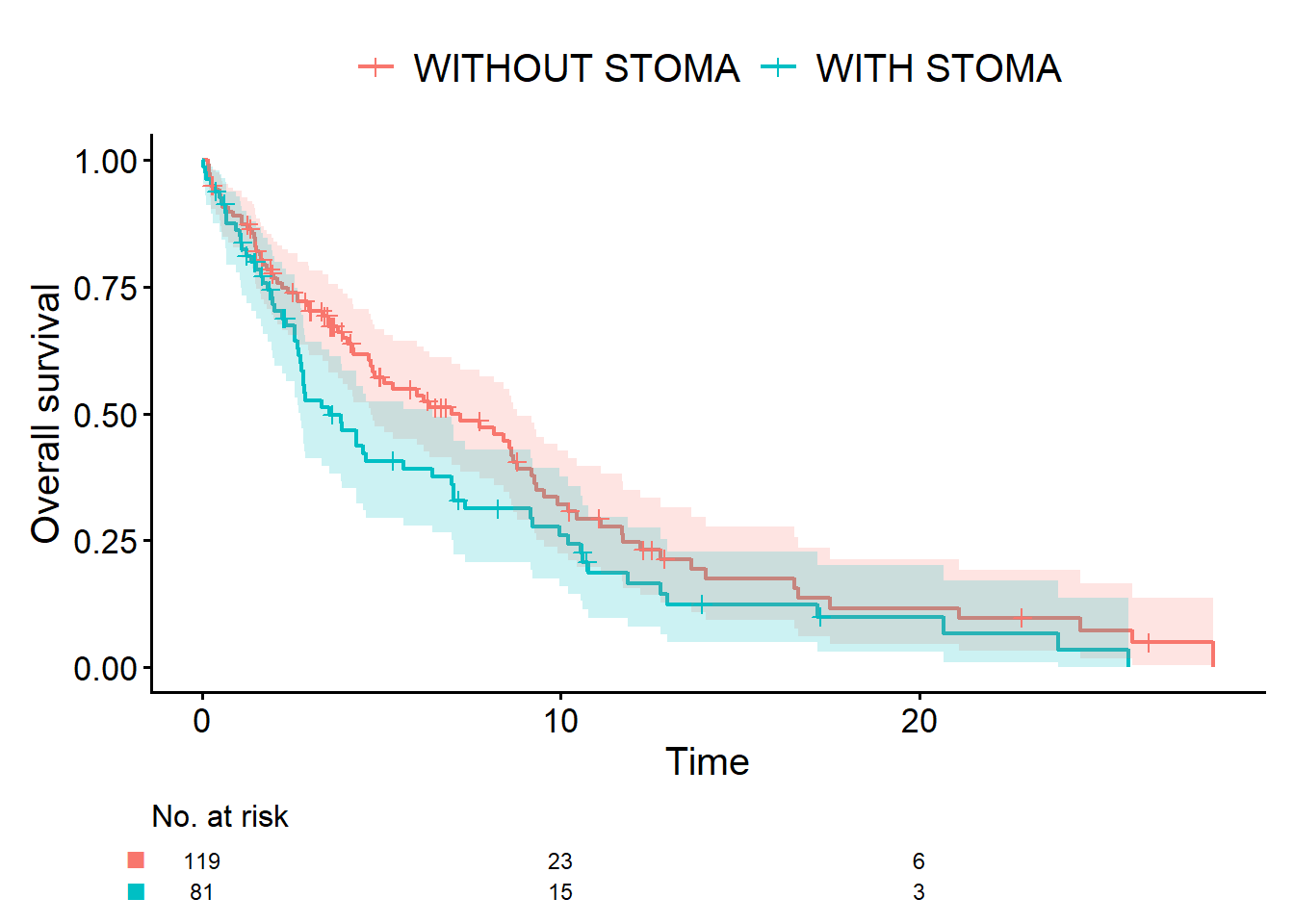
NoteKaplan-Meier curve for OS
OS and RFS are ordinary survival data, so as before we can use the cifplot() function from the cifmodeling package to draw Kaplan-Meier curves. Let us start with OS.
NoteR code and output
set.seed(46)
dat <- generate_data(hr1 = 2, hr2 = 1.5)

# devtools::install_github("gestimation/cifmodeling") # if needed
library(cifmodeling)
cifplot(
  Event(time_os, status_os) ~ stoma,
  data         = dat,
  outcome.type = "survival",
  label.y      = "Overall survival"
)
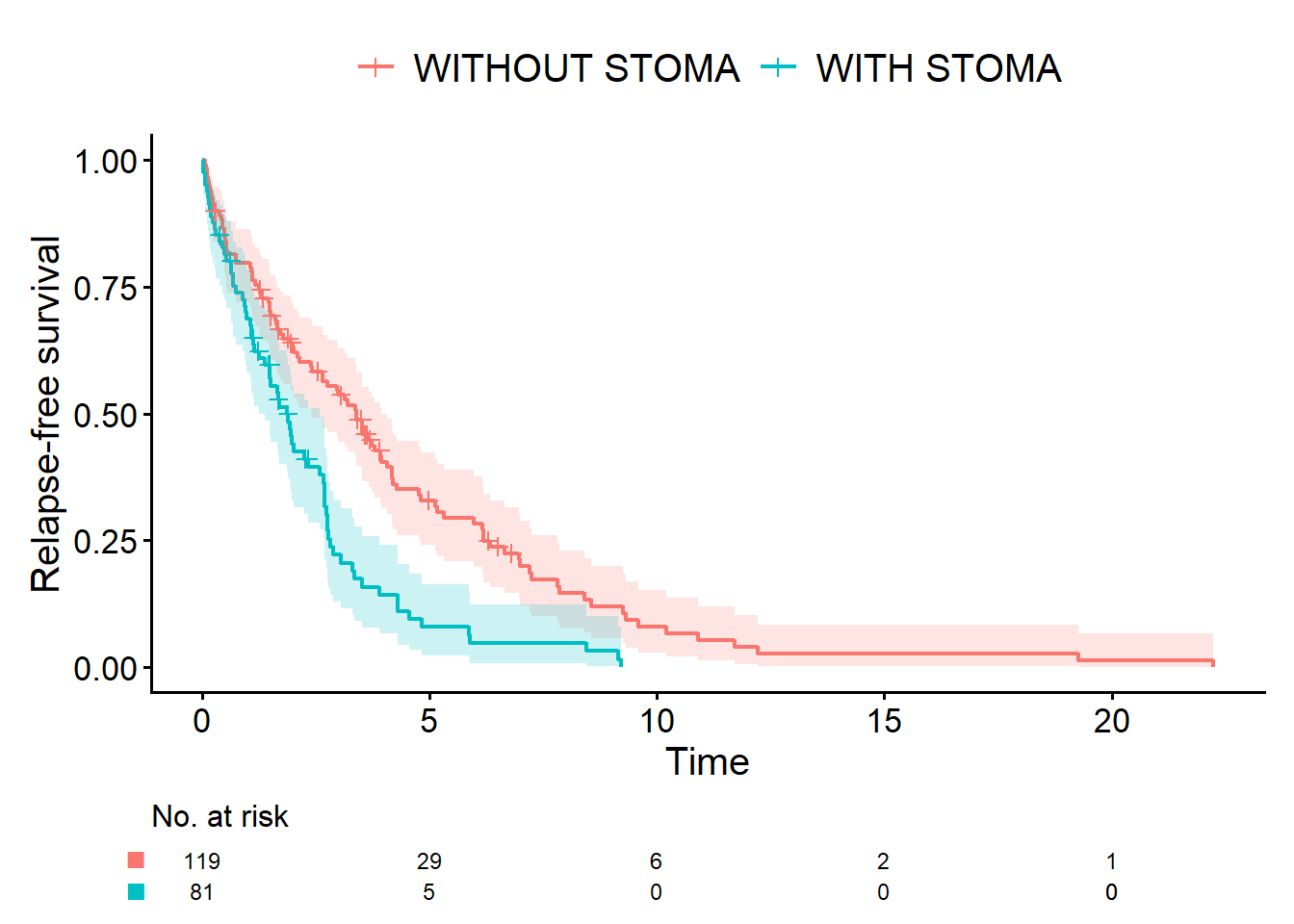
NoteKaplan-Meier curve for RFS
Next is RFS. Apart from the variables specified inside Event(), the code is unchanged.
NoteR code and output
cifplot(
  Event(time_rfs, status_rfs) ~ stoma,
  data         = dat,
  outcome.type = "survival",
  label.y      = "Relapse-free survival"
)
NoteAalen-Johansen curve for CIR
In the code below, the competing risk is encoded via Event(time_cir, status_cir):
status_cir = 1: event of interest (relapse)status_cir = 2: competing risk (death without prior relapse)status_cir = 0: censoring
By additionally specifying outcome.type = "competing-risk", we draw the Aalen-Johansen curves.
NoteR code and output
cifplot(
  Event(time_cir, status_cir) ~ stoma,
  data         = dat,
  outcome.type = "competing-risk",
  label.y      = "Cumulative incidence of relapse"
)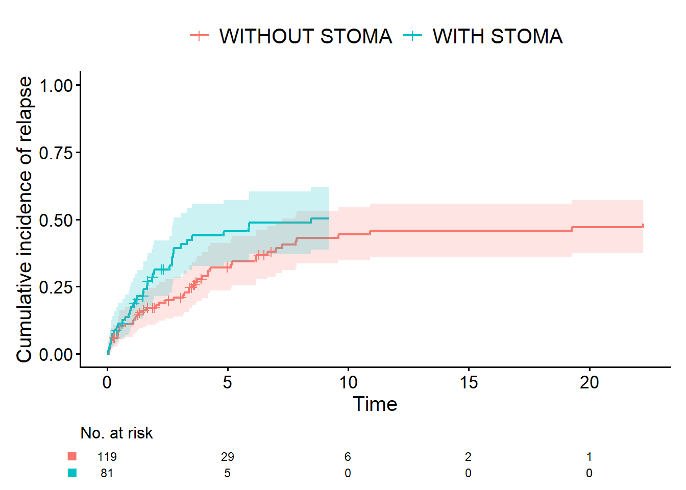
Me: “Isn’t the Aalen-Johansen curve just the Kaplan-Meier curve flipped upside down on the y-axis?”
Dad: “On the graph they can look almost identical, so it’s natural to think that. But I’d still like you to keep them distinct in your mind.
A survival curve (Kaplan-Meier) and a cumulative incidence curve (Aalen-Johansen) are different statistical procedures. When there are competing risks, you should use the Aalen-Johansen curve.
By the way, earlier you said you wanted to use ‘cumulative incidence of relapse’ rather than ‘relapse-free time’. That’s because, in technical terms, the cumulative incidence curve is synonymous with the Aalen-Johansen curve. In principle, you could analyze CIR with a Kaplan-Meier curve. In that case, deaths without relapse would be coded not as a competing risk (status_cir = 2) but as censoring (status_cir = 0). But in reality, death is a different outcome from end of follow-up or loss to follow-up. That’s why treating it as a competing risk is the appropriate approach.”
Me: “Then is it wrong to analyze RFS where both death and recurrence are treated as events?”
Dad: “No, of course not. But remember that the difference between RFS curves reflects not only recurrence but also deaths from other causes. So, as we’ve just discussed, you need to use OS, RFS, and CIR in different ways, depending on what you want to learn.”
NoteA quiz related to this episode
CDISC ADaM ADTTE (Analysis Data Model for Time-to-Event Endpoints) is a standard format for clinical trial data used by pharmaceutical companies. In this standard, the variable that indicates censoring is called CNSR. Which of the following codings represents censoring?
- CNSR = 0
- CNSR = 1
NoteAnswer
- The correct answer is 2.
In ADaM ADTTE, CNSR is the censoring indicator: 0 = event, 1 (or >0) = censored. In many R workflows, including Event() and Surv(), the default convention is event = 1, censoring = 0. You therefore cannot use CNSR directly as an event indicator.
Episodes, glossary, and R-script
- A Story of Coffee Chat and Research Hypothesis
- Data Have Types: A Coffee-Chat Guide to R Functions for Common Outcomes
- Outcomes: The Bridge from Data Collection to Analysis
- A First Step into Survival and Competing Risks Analysis with R
- When Bias Creeps In: Selection, Information, and Confounding in Clinical Surveys
- Statistical Terms in Plain Language
- study-design.R